Plotting and Post-processing
General lake information: lake.csv
The model automatically creates a file called lake.csv, that contains information about the lake volume balance, surface heat balance and other lake-scale variables that may be of interest.
Creating a custom time-series output file: custom.csv
The model can be configured to produce a time-series of any chosen variables at a custom depth. This is useful for plotting model output in Excel, R or MATLAB.
Using the in-built time-depth contour plots: plots.nml
If the xdisp command line argument is invoked, then a plot window will open and display results as the model is running. This plot window is entirely customisable, and this is done via the plots.nml text file. This file allows setting of the window size, number of plots, variables to plot, and color limits. Variables that can be plotted include: temp, salt, rad and any FABM state or diagnostic variable.
Plotting with R: glmtools
The model can be Managed within R via the GLMr and glmtools packages. Click here for the glmtools tutorial (v1.4).
Analysing the results with Lake Analyser
The model results area able to be analysed using the Lake Analyzer program developed by Read et al. (2012). In particular modellers can use this tool to compare their simulations against metrics such as thermocline depth, lake number and Schmidt stability etc. Refer to lake results for examples. MATLAB scripts to use GLM with LA are available ..here.. .
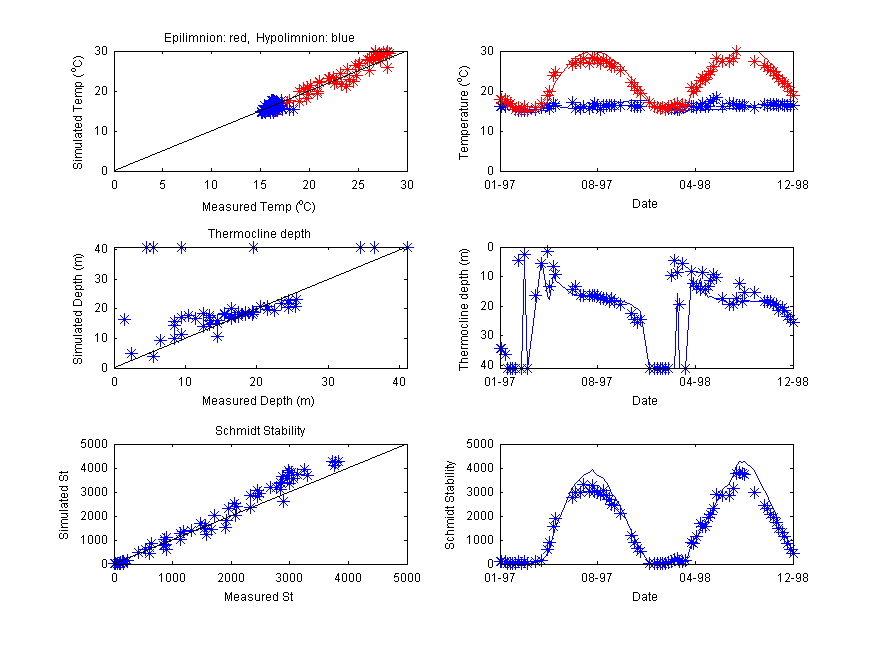
Figure 2 Overview of Lake Analyser Output
Calibrating the Model with the MCMC Tool
The model may be run with the MCMC Toolbox For Matlab in order to quantify uncertainty in model predictions. Users may run without MATLAB using a pre-compiled MCMC executable package: runMCMC
Note users will need the MATLAB R2012a MCR installed MATLAB Compiler Runtime.
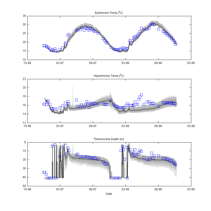
Figure 3 MCMC Output
GLM is developed as a freely available open-access tool to improve our knowledge of how changes in land-use, climate and management actions will affect our freshwater resources and lake ecosystems